MAT 152
Statistical Methods 1
The Data Table
We store data that we collect in a data table. Progames like google sheets and excel are used to create these tables.
Data tables are essential tools in research for organizing and presenting data in a clear and accessible way. They allow researchers and students alike to quickly analyze and draw conclusions from data. Here, we present a sample data table that showcases various attributes of a group of college students. The table has 5 rows since we got 5 responcese to the survey. Each row is an observation, while each column is a variable.
| Age | Handedness | Gender | Eye Color | Height (inches) | SAT Score |
|---|---|---|---|---|---|
| 19 | Right | Female | Blue | 65 | 1200 |
| 21 | Left | Male | Green | 70 | 1300 |
| 20 | Right | Female | Brown | 64 | 1150 |
| 22 | Right | Male | Hazel | 68 | 1250 |
| 18 | Left | Female | Blue | 62 | 1100 |
Describing Data
We need some key definions to describe data. In order of statistical research to meet the standards of peer review, we need to use the same definions and classifications of data. Some of the classifications are a little less strict than what is defined in our book. So, first what is a statistic?
Understanding Sample, Population, Statistic, and Parameter
Population: A population is the entire group that you want to draw conclusions about in a study. For instance, if you are studying the effects of a new teaching method, your population might be all the students at a particular university.
Sample: A sample is a subset of the population that is used to represent the population. Collecting data from a sample is more feasible than from the entire population. For example, instead of surveying every student at the university, you might select 200 students randomly to represent the whole.
Statistic: A statistic is a measure that describes a characteristic of a sample. It is calculated from the data collected from the sample. An example of a statistic could be the average test score of the students in your sample.
Parameter: A parameter is a measure that describes a characteristic of an entire population. Since it's often impractical to measure the entire population, the parameter is usually estimated through statistics from the sample. For example, using the average test score from your sample, you might estimate the average test score of all students at the university.
Categorical vs. Numerical Variables
Categorical Variables: Categorical variables represent types of data which may be divided into groups. These categories are typically qualitative and describe attributes or qualities that do not have inherent numerical values. Examples include colors of cars (red, blue, green), types of cuisine (Italian, Mexican, Chinese), or gender (male, female, non-binary).
Numerical Variables: Numerical variables represent quantities and can be measured. These can be further classified into discrete or continuous variables. Discrete numerical variables represent counts (e.g., the number of students in a class, the number of books on a shelf) and take on only integer values. Continuous numerical variables, however, can take on any value within a range and often include measurements (e.g., height of students in meters, temperature in degrees Celsius).
Understanding the difference between these types of variables is crucial for data analysis, as it determines the type of statistical analysis that can be performed. For example, you might use a bar chart to represent categorical data, while a histogram would be more suitable for numerical data. We will talk more about this in chapter 2.
Discrete vs. Continuous Numerical Data
Discrete Data: Discrete data consist of distinct, separate values where each value is individually distinguishable and countable. This type of data often involves counting, such as the number of students in a classroom or the number of books on a shelf. These are whole numbers and cannot be broken down into finer increments without losing meaning.
Continuous Data: Continuous data can take any value within a given range and are measurable. This data type involves measurements, and the range of possible outcomes can be subdivided into increasingly smaller parts. Examples include measuring the height of students, which could be any value within the range of human heights, or the time it takes to complete a task, which could be any number of seconds or minutes.
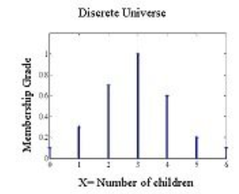
Figure 1: Since we have to have a whole number of childern, this is discrete data.
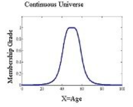
Figure 2: Since a childs age can take any real number as a value, this is continuous data.
Levels of Measurement
Understanding the levels of measurement in data collection is crucial for selecting the appropriate statistical analysis and accurately interpreting data. There are four primary levels of measurement: nominal, ordinal, interval, and ratio. Each level provides different information and has a different implication for statistical analysis.
Nominal
Nominal data are categories without any natural rank or order between them. This data type is used for labeling variables, without any quantitative value. Examples include gender (male, female, other), types of animals (dog, cat, bird), or car color (red, blue, green).
Ordinal
Ordinal data are categories with a natural order but without consistent intervals. This type of data reflects a rank or order among items. Examples include educational levels (high school, bachelor's, master's, PhD), survey responses (strongly disagree, disagree, neutral, agree, strongly agree), or economic status (low income, middle income, high income).
Interval
Interval data are numeric scales in which we know both the order and the exact differences between the values. However, this scale does not have a true zero. Examples include temperature in Celsius or Fahrenheit, where zero does not mean 'no temperature.' It allows for the measurement of the difference between items, but not the ratio between them.
Ratio
Ratio data have both a natural order and a true zero, which allows for the calculation of ratios. Examples include weight, height, distance, and duration. These measures can be doubled (e.g., one object can be twice as long as another), showcasing their ratio nature.
These levels of measurement inform the type of statistical tests that can be conducted and influence how conclusions are drawn from the data. For example, mean and standard deviation are meaningful for interval and ratio data but not for nominal or ordinal data. Similarly, one can calculate the mode for any level of measurement but median only for ordinal, interval, and ratio levels.
A quick aside: why do we need a true zero for ratio?
The zero must represent not having something. Such as 0 lbs means not having weight, where as 0 degress Celesus is just a place holder for the middle of the scale and does not mean that something at 0 degress has no temperature. If there wasn't a true zero, you could impose an arbitrary shift without changing anything substantive (as when changing Celcius to Fahrenheit, which use different zeros, both arbitrary), but then you can't make that "twice" thing make sense for either. (You can for Kelvin, though, there's a thing you actually have twice as much of.)
Now that we have a good idea of how to talk about the data we collect, let's look at how we actually collect the data.
Getting and explaing data
from Studies or Experiments
As stated before, if you want to know something about a population, it is often impossible or impractical to examine the whole population. There are many ways to collect a sample, and we hope to use good sampling practices to insure that the sample behaves the same as our population.
Observational studies vs controlled experiments
There are two main techniques to systematically collect data:
- Observational studies and
- Controlled experiments
Observational studies
An observational study is one where the data collection does not interfere with how the data arises. Examples include
- Surveys,
- Review of records,
- Simple measurements
Sampling Methods
Choosing the right sampling method is crucial for research because it significantly affects the validity and reliability of the results. Here are five common sampling methods used in data collection, each suited for different types of research scenarios.
Simple Random Sampling
Simple Random Sampling is the most basic form of sampling. Every member of the population has an equal chance of being selected. This method can be implemented using lottery methods or computer-based random numbers. Example: Selecting 100 students from a school’s enrollment list using a random number generator.
Systematic Sampling
Systematic Sampling involves selecting members from a larger population according to a random starting point but with a fixed, periodic interval. This method is often easier to conduct than a simple random sample. Example: Choosing every 10th visitor entering a mall from a list of all visitors.
Stratified Sampling
Stratified Sampling divides the population into smaller groups, or strata, based on shared characteristics. A random sample is then taken from each stratum. This method ensures representation from all segments of the population. Example: Dividing a university’s student body by major and selecting a random sample from each major to assess career preferences.
Cluster Sampling
Cluster Sampling is used when natural groups are present in a population. The entire population is divided into clusters, and a random sample of these clusters is chosen. All individuals within the selected clusters are surveyed. Example: Researching community health trends by selecting random neighborhoods (clusters) and surveying every household within them.
Convenience Sampling
Convenience Sampling involves selecting a sample from parts of the population that are conveniently accessible. This method is less reliable and is not representative of the entire population, but it is the quickest and easiest method. Example: Interviewing people who pass by a certain street corner at a certain time of day.
Each sampling method has its advantages and limitations, affecting the research’s scope, resources, and objectives. Understanding these methods helps in choosing the most appropriate one to meet the specific needs of a study.
Controlled experiments
In an experiment, researchers actively work with the samples applying treatments and observing effects.
- Often (if not always), the intention is to explore a relationship or even a causal effect between two variable.
- For that reason, it's often important to distinguish between an explanatory variable and a response variable.
An observational example
Suppose we are interested in the following question:
Does caffeine consumed through coffee affect GPA among CCCTI students?
The observational approach
To perform an observational study, we might select 14 CCCTI students and interview them. We might ask a number of questions but two questions key to the study would be:
- How much caffeinated coffee do you drink (in cups)?
- What is your GPA?
The resulting data
If we interview 14 of the 3876 students at CCCTI, we might generate a table that looks something like so:
| ID |
Daily Coffee intake (cups) |
Current GPA |
|---|---|---|
| 1 |
2 | 4.0 |
| 2 | 1 | 4.0 |
| 3 | 1 | 4.0 |
| 4 | 4 | 3.8 |
| 5 | 2 | 3.3 |
| 6 | 3 | 3.1 |
| 7 | 2 | 2.8 |
| 8 | 4 | 3.1 |
| 9 | 7 | 2.3 |
| 10 |
0 | 3.1 |
| 11 | 1 | 4.0 |
| 12 | 4 | 1.8 |
| 13 | 2 | 2.1 |
| 14 | 3 | 3.7 |
Visualization
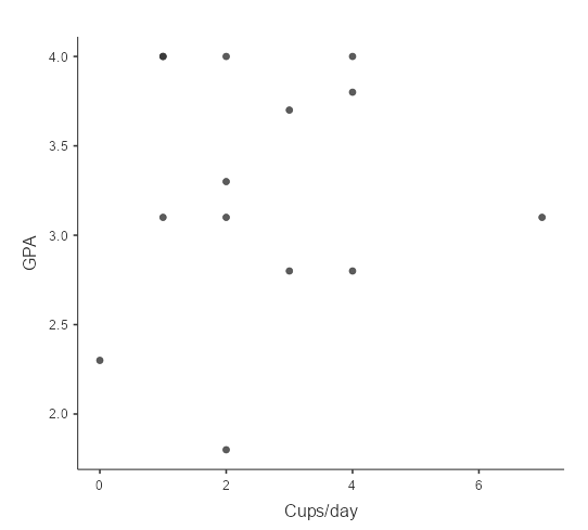
We might visualize the data with a scatter plot.
Analysis
The numbers and picture kinda appear to support the idea that caffeinated coffee consumption improves GPA. Of course, we ultimately hope to be able to quantify that type of analysis more precisely.
Sample/population for the coffee example
In the coffee example (where we interviewed 14 of the 3876 students at CCCTI),
- The sample is the 14 students we interviewed.
-
The population is the set of all 3876 CCCTI students.
(The extent to which the conclusion might extend to all college students anywhere might be a point of discussion and further research.)
Statistic/parameter for the coffee example
Suppose we find that, of the 14 students in our sample, the students drink 2.57 cups of coffee a day on average.
- That average number 2.57 computed from the sample is a statistic.
- If we could somehow determine the average number of cups of coffee consumed by all 3876 CCCTI students, that number would be a parameter.
Typically, it's not necessarily feasible to compute a parameter from an entire population. Thus, we estimate population parameters from sample statistics. A key question is:
How close can we expect a computed statistic to be to the corresponding population parameter?
Some important issues
- Confounding variables
- Causation vs correlation
Confounding variables
A confounding variable is a variable (often unknown) that influences two or more other variables and causes a spurious association.
In the coffee GPA example, a confounding variable might be the amount of time the student studies. If they study a lot, the might find themselves drinking more coffee and increase their GPA.
The term lurking variable is a synonym for confounding variable.
Causation vs correlation
In statistics, we are often interested in the effect of one variable on another. In the context of the coffee study - does the consumption of caffeinated coffee improve GPA?
Due to the potential presence of unknown confounding variables, whether there is a relationship between two variables - and not whether there is a causal relationship.
This is sometimes phrased as
correlation does not imply causation.
To establish a causal relationship, you've really got to set up and experiment.
An experimental example
In an experiment (more specifically, a controlled experiment), researchers actively work with the samples applying treatments and controls and observing effects.
Let's outline an experimental approach to our another GPA question:
Does 8 or more hours of sleep each night affect GPA among college students?
The experimental approach
To explore this question via a controlled experiment, we would start with a large, simple random sample of participating college students. We would randomly assign the each student into one of two groups:
- The treatment group, who would be required get 8 or more hours of sleep each night and
- the control group, who would get less than 8 or at least they are not required to get 8 hours.
After some pre-specified amount of time, we would check and compare the grades earned by the two groups.
Results
If there were 250 participants in our sample, perhaps our results might look something like so:
| Treatment | Control | |
|---|---|---|
| N | 119 | 131 |
| GPA | 3.7 | 2.9 |
This looks like it might be compelling evidence that 8 hours of sleep boosts GPA. We would ultimately like to be able to quantify that statement.
Some key principles of experiments
-
Control: We split the group of patients into two groups:
- A treatment group that receives the treatment
- A control group that receives a placebo.
- Randomization: The groups should be chosen randomly to prevent bias and to even out confounding factors.
- Replication: The results should be reproducible
If we find differences between the groups we can examine whether they are statistically significant or not. We will cover this idea in more detail in unit 3.