What are discrete random variables?

Remember that a random variable, $X$, is derived from a random process with some numerical outcome. Our book notes that "In many cases the random variable is what you are measuring, but when it comes to discrete random variables, it is usually what you are counting." (p. 157) So, let's look at some examples to make this clear what we mean by discrete random variables.

• Example 1: Choose $X$ to be the sum of the scores of the next 5 Steelers home games
• Example 2: Filp a coin and write Down
  • $X = 1$ if the coin lands on heads
  • $X = 0$ if the coin lands on tails
• Example 3: Let X be the size of a household in the US in 2023. That is the number of current residents.
• Example 4: Let X be the number of cylinders a car's engine has.

All these examples only produce integer values. In the language of probability theory that we developed last week, we would say that the sample sapce is the set of integers

Distributions for discrete random variables

Our book says, "A probability distribution is an assignment of probabilities to the values of the random variable" (p. 157).

The book uses a good example from the 2010 US Census as seen below:

Note that all the probabilities should be non-negative and they should add up to one. For a discrete random variable, the distribution is created by listing out the probabilities that the random variable has for each specific value. Such as there being a 0.336 or 33.6% probabily a house randomly selected from the census would have $2$ members living in it.

Functional notation

We will also see that information from the chart displayed in functional notation. For example we could list some values from the previous table:

• $P(X = 1) = 0.267$
• $P(X \geq 7) = 0.015$
• $P(X > 3) = 0.137 + 0.063 + 0.024 + 0.015 = 0.239$ or about 23 percent

What about the Mean of the distribution?

The mean or expected value of a discrete random variable $X$, symbolized as $E(X)$, is often referred to as the long-term average or mean (symbolized as $μ$). This means that over the long term of doing an experiment over and over, you would expect this average. The mean of a discrete distribtuion is calculated using the folloing formula

In our household example we could get a mean

Note that we had to extimate 1.7% to be close to 7, so our 2.5 is an underestimate.

Pictorial representation

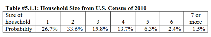
A fianl way to represent a discrete distribtuion is with a a plot that looks like a histogram:

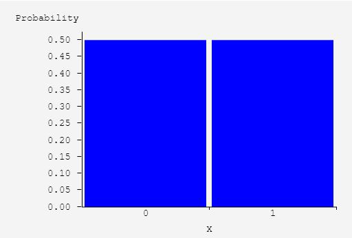
The graph of the left can represent a fair coin flip, what about the one on the right?

This represent the distribution for X ~ 1 if an adult over 20 has a caviety, otherwise 0. (SOURCE)

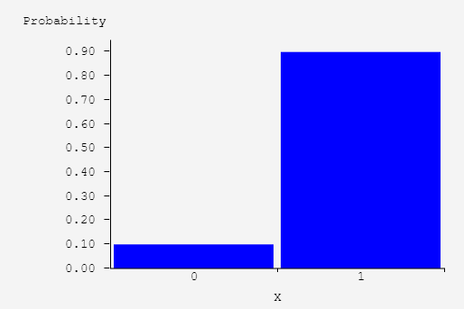
The discrete, uniform distribution

If the sample space of a discrete distribution consists of $n$ consecutive integers, each of which has probability $1/n$, then the distribution is said to be uniform. For example we might look at a 6 sided die:

We can look at the graph:

The roll of a six-sided die or the flip of a coin can each be represented with a discrete uniform distribution.

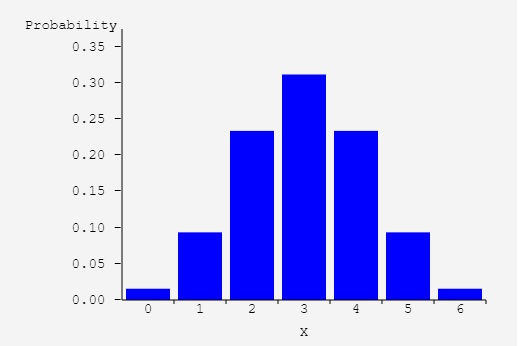
What about discrete, non-uniform distribtuions?

Notice how this is different from our uniform distribution. If this were a distribtuion for a 6 sided die, which number do expect to come up the most

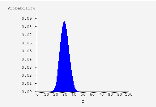
Pictorial representations of discrete distributions make particular sense when there are a large number of possibilities. The image portrays a discrete distribution where the sample space is the set of integers between 1 and 100 and smaller numbers are more likely to be chosen than larger numbers.

Properties of a Bernoulli trail

Now we are going to look at Bernoulii trials (binomial experiments), so that we can better understand the binomial distirbution. First we want to be able to recognize when we have a Bernoulii trail. Here are some key concepts to look for in identifying a binomial experiment:

Fixed number of trials, $n$, which means that the experiment is repeated a specific number of times.

The $n$ trials are independent, which means that what happens on one trial does not influence the outcomes of other trials.

There are only two outcomes, which are called a success and a failure.

The probability of a success doesn’t change from trial to trial, where $p$ = probability of success and q = probability of failure, $q = 1-p$.

The binomial distribution

If you know you have a binomial experiment, then yuo can calculate binomial probabilities. When you list these out in a table or graph you have created a binomial distribton.

The binomial distribution is a discrete distribution that plays a special role in statistics for many reasons. Importantly for us, the binomial distribution allows us to see how a bell curve (in fact the normal curve) arises as a limit of other types of distributions.

Looking at an example:

This example come from the book on page 170 - 174. I will be using this calculator but you are free to use which ever calculator you want. Desmos can help with both the formula and the direct calculation and has a simular imput command as the ti-84.

When looking at a person’s eye color, it turns out that $1$% of people in the world has green eyes ("What percentage of," 2013). Consider a group of $20$ people.

• State the random variable.
• Find the probability that none have green eyes.
• Find the probability that nine have green eyes.
• Find the probability that at most three have green eyes.
• Find the probability that at most two have green eyes.
• Find the probability that at least four have green eyes.